Bridge Modeling F.LE.A.1

CCSS.MATH.CONTENT.HSF.LE.A.1

Distinguish between situations that can be modeled with linear functions and with exponential functions.

The Problem:

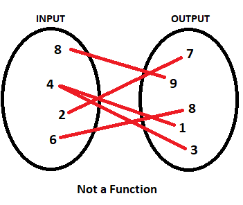
We begin the lesson with introducing (or reminding) students of the concept of a function. For the purposes of this lesson, we will define a function as an expression containing one or more variables in which each input has one and exactly one output.


It is also understood that before continuing with the lesson, students are aware of at least the basic shape of some basic graphs: linear, quadratic, polynomial, exponential, logarithmic, and sinusoidal.


Once the understanding has been established, we introduce the lesson objective to the students: for them to create a functional model for determining the breaking weight of paper bridges by predicting a best-fit graph.


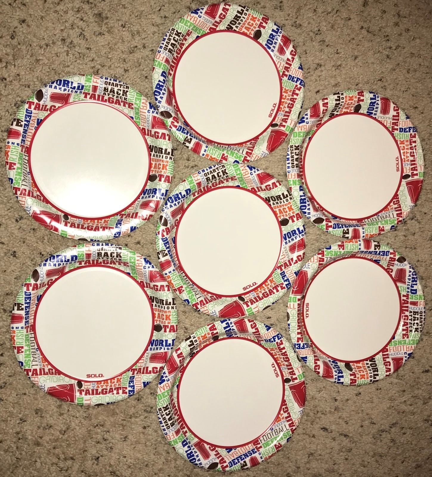
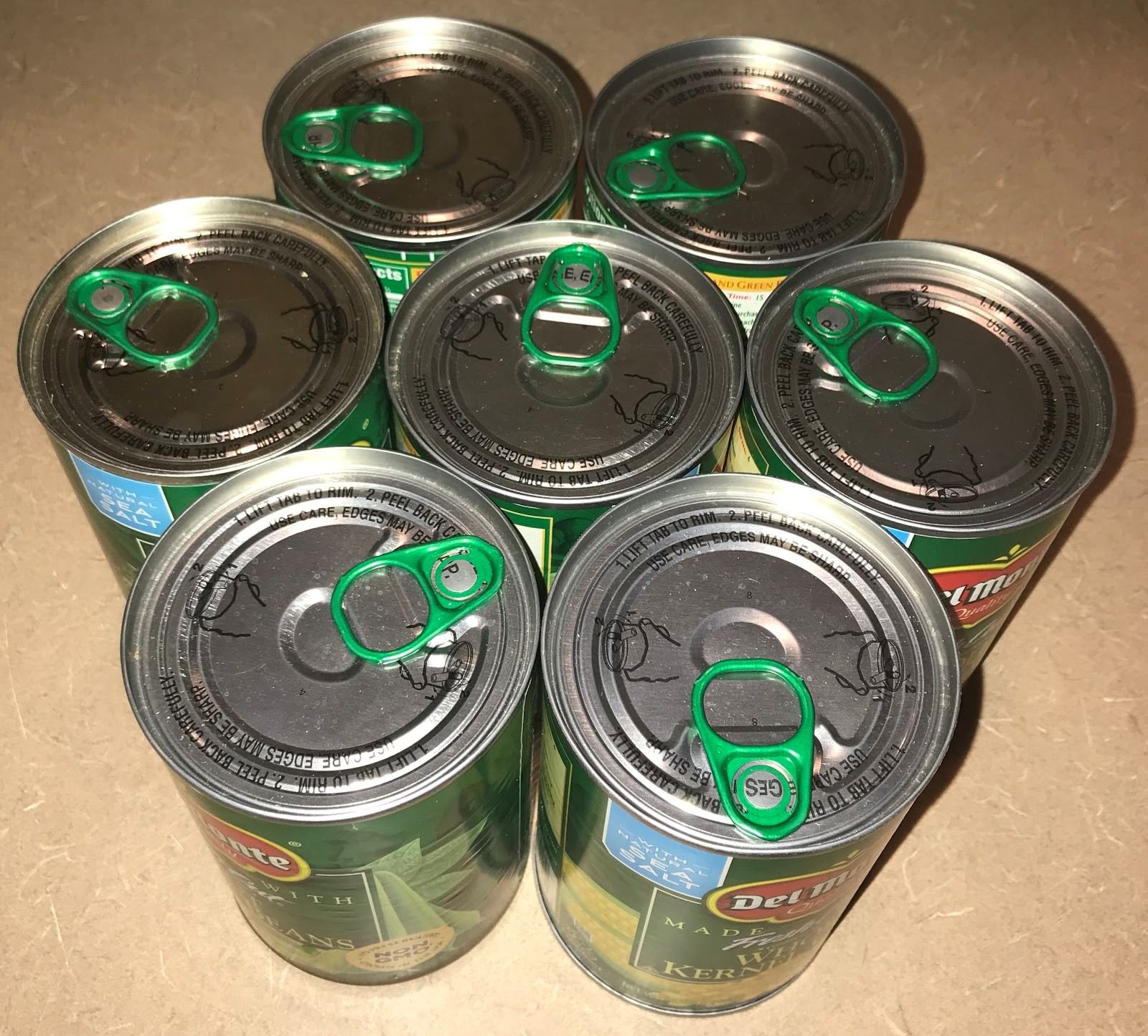
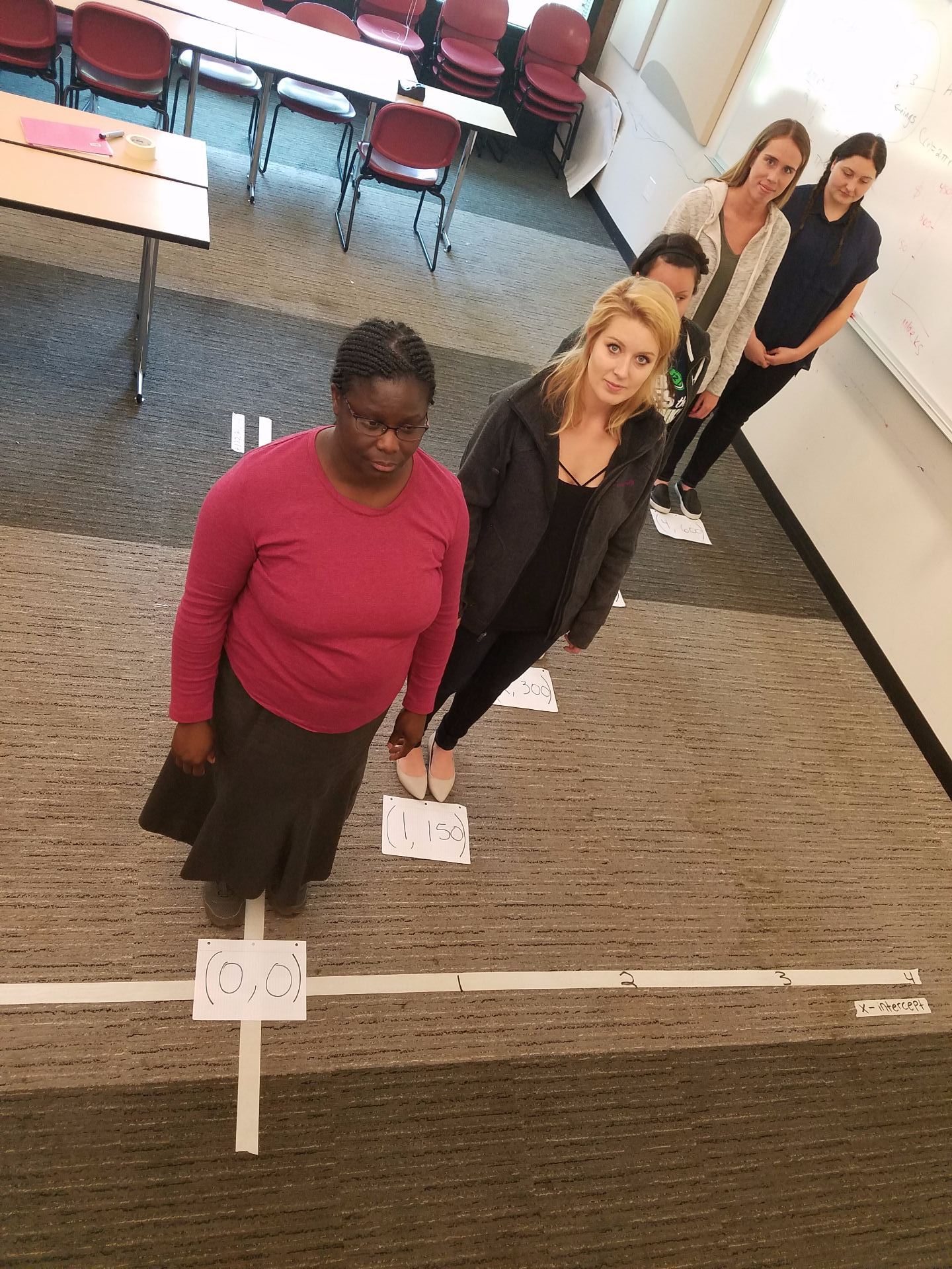
To complete their task, students are given at least 10 strips of paper measuring 11”x4”. They will also require about 40 pennies, as well as two books of about the same thickness. Students will make a one inch fold along both of the long sides to create a bridge, then suspend their bridge between the two books, as shown below.

Students will then stack pennies on their bridge. Eventually their paper bridge will fall, and students will record the number of pennies their bridge was able to hold before falling. Once that number is recorded, that paper bridge is “retired”. Students will then take two strips of paper stacked on top of each other, create the same 1-inch fold along both of the longer sides, and suspend their new 2-layer bridge between the books. Students will again begin stacking pennies on their paper bridge, recording the number of pennies their bridge was able to hold when it falls. They will continue their process for 3 layers of paper, as well as at least 4 and 5 layers but continuing to as many layers as desired.


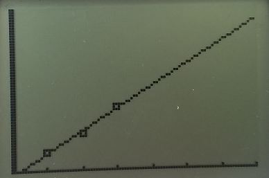
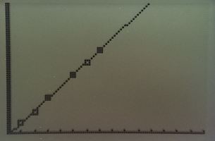
Once the data has been collected, students will use their calculator to input the values into the scatterplot and analyze their graph to determine a best-fit equation.


Our Approach:

Our experiment went well for our first three trials, that is the 1, 2, and 3 layer bridges. We found that for the 1-layer bridge we were able to hold 8 pennies. The 2-layer bridge held 16 pennies and the 3-layer bridge held 27. The difference between the first two values is 8, while the difference between the last two is 11. The differences are close enough that it could suggest a linear regression, although with three points it is hard to tell, and we concluded further testing was required.


Our fourth trial resulted in a paper bridge capable of withstanding 68 pennies. This was a difference of 41 from the 3-layer bridge, and threw our theory of a linear regression out the window. We went back to the differences between the first few data points, and although the differences were similar we realized the first difference is smaller than the second difference. We used a calculator to plot the four points, and to create an exponential regression.


However, we were hesitant to accept this result. Was our outcome for the 4-layer bridge a fluke, or a statistically significant event? We continued creating and testing 5, 6, and 7 layer bridges, and found that they were able to hold 45, 55, and 65 pennies, respectfully. The consistency of differences immediately told us that we are not, in fact, dealing with an exponential function. We went back to our original idea of a linear function, excluding our 4th trail’s data completely.


Because of our uncertainty, we decided to determine our margin of error. We used the equation for our linear function to “predict” what our outcome should have been for the 1-3 and 5-7 layer bridges, and we determined as follows: 

Trial # # of pennies bridge held # of pennies bridge should have held (following linear equation) Difference
1 8 7.5 .5
2 16 17 1
3 27 26.5 .5
5 45 45.5 .5
6 55 55 0
7 65 64.5 .5

By adding the differences and dividing by 6 (our number of data points), we get our average difference between the points and the linear regression line of 0.5. This means that we could estimate the number of pennies a 100-layer bridge could withstand, and our number would be accurate within ½ of a penny.

Circles and Squares 7.RP.2.a, 7.G.A.1, and 7.G.B.4 MP 4

Circles and Squares

Standard: CCSS.7.RP.2.a CCSS7.G.A.1 CCSS.7.G.B.4 Math Practice 4

By: Naomi Johnson, Rachel Van Kopp, Tracy Van Lone, Natasha Smith, and Kimberly Younger

The problem:

This problem was based on Circle-Square by Dan Meyer and had a circle and a square on a line that moved together. When one shape grew, the other would shrink by the same amount. Our job was to find out when the two shapes would be equal in area.

Connections/Solution:

We found that when the perimeter of the square is 21.1 and the circumference of the circle was 18.9, then the areas would be equal to each other. After finding the areas, we noticed that the equations for the two were very similar. The area for the square was A = 28.4234 and the area of the circles was A = 28.4234, so the square was divided by 16 and the circle was divided by 12.567, so the radius of the circle and the distance from a corner to the center of the square will be very close. Another connection that we noticed was that their perimeter and circumference will always equal 40 because that was the length of the number line it was on.


Extensions:

  1. Have the circle and square not touch, and looking at how that might change the perimeter and circumference. They could also extend the number line from 40 to 60 or beyond and looking at the impact that would have. For discussions, the teachers could have the students think about what would happen if, instead of the two shapes moving together, they moved apart from each other.
  2. Use a cube and sphere instead of a circle and square:

    Sphere & Cube Dimensional Relationship Exploration

    What are the dimensions of a cube and a sphere of equal volume?
    What are the dimensions of a cube and a sphere of equal surface area?
    Are there any cool relationships between the dimensions of the cube and the sphere?
    Which cube dimension most closely resembles the sphere’s radius? Why?
    Use these calculators to analyze the relationships:
    Cubehttps://www.geogebra.org/m/g6ffapbP    Spherehttps://www.geogebra.org/m/Xyc8W4Qn

(Note: The sphere radius illustrated above is 1/phi. The cube edge is 1.)


Kissing Coins 7.G.A

Kissing Coins

BY: Jessi Smith, Paloma Vergara, Kaitlin Brame, and Bailey Martoncik

The problem:

For this activity, Dr. Oursland gave each table 7 poker chips. Each poker chip is uniform in size. We were asked to organize the poker chips in a circle kissing a center chip (see visuals). Next, we were asked to predict whether or not this unique kissing relationship will work for all uniform circular objects. Then we tested our hypothesis with another set of 7 uniform circular objects. Then we drew the problem and looked at the connections between the radius, diameters, triangles, and regular polygons to help prove that this kissing relationship will work for all uniform circular objects.

What we did and the connections we made:

Once we had the circular objects (poker chips and flip coins) in the seven coins circle “kissing” one another, we drew what we saw and then discussed in our group what we saw and why we thought that the “kissing coins” arrangement worked for similar circular objects. The first thing discussed was that all the circular objects had the same circumference, radius, and diameter. This discussion furthered to how if you measure from one circle to the center of a circle that it is “kissing” you get the length of two radii which is the length of one diameter. We quickly realized that connecting the centers of circles created six equilateral triangle or one hexagon. The diagonals on this hexagon is equal to four radii or two diameters. After some discussion, we concluded that this arrangement would work even if we scaled the objects up or down in size.

Application:  

The Kissing Coins activity can be applied in the classroom by having students evaluate various circular objects with same radius and comparing what they see in terms of shape connections. For example, when students draw a representation on graph paper using the seven circular objects, they will be able to start identifying other shapes like trapezoids, equilateral triangles, hexagons, scalene triangles, and rhombuses. Students will be able to make these connections and more with this activity. The Kissing Coins activity can also be used with Common Core State Standard, 7.G.A.3 which states, “Draw, construct, and describe geometrical figures and describe the relationships between them”. Students can begin with the circle and then begin to make connections about the relationships between shapes. The activity or lesson could be extended further by having students compare the circumference of a circle to the perimeter of a rectangle. In addition to State Standards, the Kissing Coins activity aligns with Mathematical Practice 4 and 5. Students can model with mathematics and use appropriate tools strategically by demonstrating the relationships between shapes using diagrams and using manipulatives and rulers to draw their representations to scale. Overall, the Kissing Coins activity is a rich task that is accessible to all students and can be modeled using a variety of objects including everyday items such as coins, coffee cups, donuts, wheels/tires, trash cans, canned goods, jars, and so on.


Kissing Coins: The Hexagonal Unit Circle 7.G.A, 7.G.B, & HSG.CO.C

KISSING COINS 

By Rachel Van Kopp, Kimberly Younger, Tracy Van Lone, Natasha Smith, and Naomi Johnson

7 chips are arranged to kiss (touch) each other.

The chips are connected to each other and look similar to a flower.

What if the coins were different sizes?

The chips are still connected in the same pattern.

After sketching a picture including all seven chips it quickly becomes a parent that there are 6 lines of symmetry. 3 of the lines of symmetry go through the center of two circles. after connecting all of the circles’ center points it is easy to see 6 triangles and 1 hexagon.

Proof – That the radius of the center circle is equal to the six outside circles. The proof is below.


The connection between circles, triangles, and regular polygons is an important part of why the circles of all the same sizes touch. The proof shows that the center points of 3 circles will create a triangle with a 60 degree angle. If you add on an additional circle your angle will be 120 degrees. Add another circle and the angle will be 180 degrees, add another circle and the angle will be 240 degrees, and adding another circle will be 300 degrees. The proof is related to the standard CCSS.CONTENT.MATH.8.G.A.5 because the standard is discussing equilateral triangles and the cos proof we used is based off of an equilateral triangle.

Extension:

Teachers can expand on sphere packing and what the packing number would be at different dimensions, i.e. how many spheres in a 3D packed space. Teachers can expand with unequal sphere packing, which would be spheres with different radii. Or another extensions could be adding layers onto the original circles and figuring out how many circles will fit on the third or fourth layer

(Follow this link to the video.)

Click the image below to watch a GeoGebra Video about Hexagonal Circle Packing.


Shape Sorter Activity CCSS.Math.Content.6.SP.B.5.b

By: Nick Spencer, Sam Marcoe, Grayson Windle, Elizabeth Englehart

With the Shape Sorter activity, which can be located at this website, we enable our students to work with several different concepts such as venn diagrams and geometric patterns.  The students work with a venn diagram in which they can set up two “rules” for each side of the diagram, and then are tasked with organizing the shapes accordingly to the rules.  If a shape meets both standards set by the rules, the student can place the shape in the center of the venn diagram, and if the shape doesn’t meet the criteria for either rule the student can leave it outside of the venn diagram.

In the figure above, my group of teacher candidates created our own venn diagram with these two rules:

  1. The figure has at least one line of symmetry (left side)
  2. The figure has rotational symmetry (right side)

In the beginning of this activity, we have several different shapes and begin organizing them in the matching part of the venn diagram based on their geometric characteristics.  The figures on the left side of the diagram have at least one line of symmetry while the figures on the right have rotational symmetry.  The figures in the center have both characteristics set by our rules, while the figures on the outside have neither lines of symmetry nor rotational symmetry.

This online educational activity allows the students to further develop conceptual understanding, and practice procedural fluency for geometric shapes and laws, as well as develop understanding for venn diagrams.  By allowing students to combine geometry with venn diagrams, students can open their perspective that venn diagrams can be utilized in various and unique situations.


Coke V. Sprite CCSS.Math.Content.6.RP.A.3

In Dan Meyers Coke V. Sprite activity, found on http://mrmeyer.com/threeacts/cokevsprite/, students use both mathematical concepts and logic principles to develop an argument. The student defends their position by organizing their reasoning, then communicating a compelling argument with their peers. Students are asked to use several representations when presenting the problem, this allows students to eventually get a better understanding for how to use mathematical procedures related to ratios.

When we completed this task as a group we determined that is was necessary to give a hypothetical amount of equal proportions of the respective sodas in each glass. We then took the dropper of Sprite and mixed it with Coke. This causes a change in the ratio (or concentration) between the amount of Coke and Sprite compared to the whole. We now proceed in solving the ratio in terms of percentages. Taking the amount of Coke and dividing it by total amount of soda, we end up finding that 90.9% of the liquid is Coke and 9.1% is Sprite.

We now take our new mixture and add it to our untouched Sprite. First, we must find out how much of the sample is Coke and how much is Sprite. By using the percentages, we found of the Coke and Sprite mixture, we multiply to find the amount of each soda within the sample.  In conclusion, both glasses contain an equal amount of their respective contents. The Sprite with Coke was 90.9% Sprite and 9.1% Coke. The Coke with Sprite was practically the reciprocal of the Sprite with Coke, 90.9% Coke and 9.1% Sprite.

This activity could be covered in a 6th grade math class towards the end of their study of ratios and proportional relationships (CCSS M 6.RP 3.c.) to help the students understand percentages, and how to use percentages in a situation where they need to understand what ‘100%’ of something is that isn’t directly given as 100 units, for example. This might be quite complex for this level, however, and could also be used as a lesson for 7th grade students (CCSS M 7.RP 3.) where the students are to be expected to solve problems with multiple steps.

Will this lemonade stand function? 8.F.B.4, 8.F.B.5, MP4

Students engage in a real world application of linear functions when they are asked to help Jimmy find the break-even point for his lemonade stand. This is a summative project based learning assignment that will push students to deepen their conceptual understanding of linear functions about real world applications. This lesson is designed for an 8th-grade class modeling linear functions and their graphs. The students will be working in small groups to help Jimmy find his break even for the lemonade stand using linear functions and their graphs.

Lemonade Stand Lesson Plan final-1k9ykd7

Meatball Problem: Content.8.G.C.9, Practice.MP4

The central focus of this learning segment is to provide an opportunity for students to model and solve a real-world mathematical problem related to the volume of different 3-D shapes. In this lesson, students will use the formulas for the volume of a sphere and volume of a cylinder to help them answer the guiding question, “How many meatballs will it take to completely fill this plastic container with sauce?” Students will then have an opportunity to put theory into practice by actually modeling the problem and testing their answers to see if they were correct. As students work to solve the problem they will provide written and oral responses to justify their work and through their responses, it is expected that it will be made explicit by the students how and why they used certain volume formulas to find their answer.

Meatballs-183grpn

Math 486 Lesson Plan-27przez

You Bakin’ Me Crazy with these Functions! 8.F.B.4, 8.F.B.5, MP.4

Students dive into the food industry when they are asked to design their own Food Trucks. A summative project based learning assessment will challenge students to analyze the importance of functions in the real-world. This is an eighth grade modeling lesson with linear function models and graphs. Students will be working in groups on their journey of creating a multi-variable function and visually represent as well as connect through a graph.


You Bakin’ me Crazy with these Functions Lesson-14f6nkp