COWculating – Picture Problem 8.F.B.4

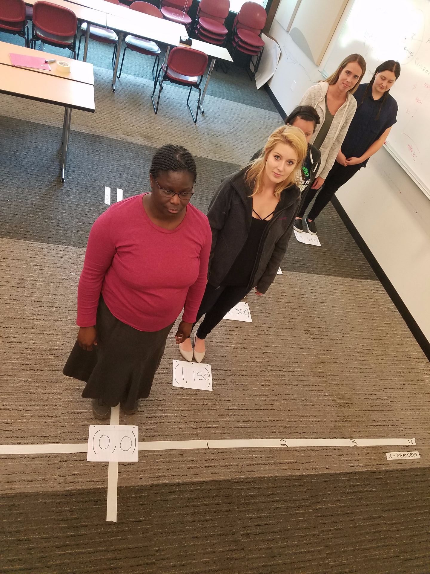
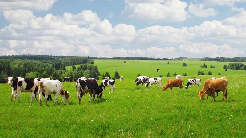
This picture – taken from Freedom Works UK – becomes the center of a fun and highly interactive mathematics lesson where students get to think what it might be like to be a farmer! Students will be assigned a set number of cows that eat a set square footage of grass per day, and must determine how much land is needed in order to sustain the cows. Furthermore, students must consider the amount of time needed in order for grass to grow back, but they must have enough already grown for the cattle to eat in the meantime.

This lesson has students focus working on the Common Core State Standards:

CCSS.MATH.CONTENT.8.F.B.4
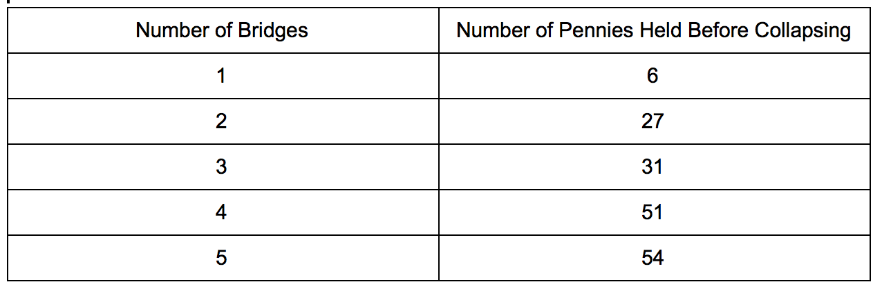
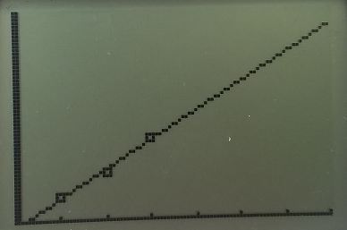
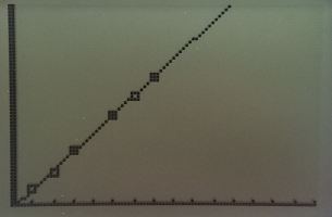
Construct a function to model a linear relationship between two quantities. Determine the rate of change  and initial value of the function from a description of a relationship or from two (x, y) values, including reading these from a table or from a graph. Interpret the rate of change and initial value of a linear function in terms of the situation it models, and in terms of its graph or a table of values.

CCSS.MATH.CONTENT.8.F.B.5
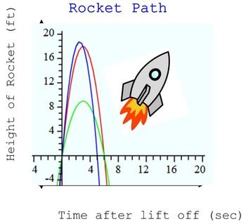
Describe qualitatively the functional relationship between two quantities by analyzing a graph (e.g., where the function is increasing or decreasing, linear or nonlinear). Sketch a graph that exhibits the qualitative features of a function that has been described verbally.

CCSS.MATH.PRACTICE.MP2
Reason abstractly and quantitatively.

Mathematically proficient students make sense of quantities and their relationships in problem situations. They bring two complementary abilities to bear on problems involving quantitative relationships: the ability to decontextualize—to abstract a given situation and represent it symbolically and manipulate the representing symbols as if they have a life of their own, without necessarily attending to their referents—and the ability to contextualize, to pause as needed during the manipulation process in order to probe into the referents for the symbols involved. Quantitative reasoning entails habits of creating a coherent representation of the problem at hand; considering the units involved; attending to the meaning of quantities, not just how to compute them; and knowing and flexibly using different properties of operations and objects.

This lesson correlates to the culture of the Ellensburg area, for a large portion of this area is populated by those in the agricultural profession. While most of them are in the hay production/distribution realm, students could connect to this rural lesson nonetheless.

World Population [Picture Problem] 8.F.B.5, L.8.3, and MP.1

By: Kimberly Younger

This image of the world, from World Mapper is skewed based off the current population in each country. Students will be assigned a country and will be asked to find out the population of the country in 1918 and the current population (2018) then they will compare the the change in population.

The lesson will focus on the standard CCSS.Math.Content.8.F.B.5 which is finding the functional relationship between two quantities, whether they are increasing or decreasing and for the this lesson they would be focusing on only linear functions. The lesson will be called Population Change Project, students will sketch the graph with the population data they collect and write a paragraph about the data the collect and interpret what it means. Including information about why they think the population increased or decreased.

This Lesson is culturally responsive because students will be learning about other countries and why the population may have increased or decreased over decade (1918 – 2018). Students could be supplied with websites which show the current population and the passed population or they can be given time to do the research on their own.

The students will use the mathematical practice of CCSS.Math.Practice.MP1 which focuses on students problem solve and preserve in solving math problems. CCSS.ELA-Literacy.L.8.3 is the use knowledge of language and its conventions when writing. The evidence of this standard would be found when students complete their write up about the change in population over the passed decade.

Disneyland Drive! – 8.F.B.4, 8.F.B.5

Students are put to the test in this fun and highly interpretive summative review of the previous unit: linear functions!

You and your family are going on a trip to Disneyland, but you must drive there! Your parents have decided that they don’t want the wear-and-tear of such a trip on their own vehicle, so they have narrowed it down to two (2) rental vehicles. However, they are having a hard time figuring out which one would be the most efficient/economical choice. Your job is to gather all the information you can, and construct a minimum of five (5) equations, graph them on GeoGebra, and lastly must decide which car your parents should choose for your vacation!

In order to complete this lesson, students will be split into groups of 3-5 members. The class as a whole will have a set gas price, but each group will have different vehicles as well as a monetary cap that they must remain under.

ModelingLessonPlan

Rocket Math: 8.F.A.3, 8.F.B.5, MP4


Rocket Math

By: Natasha Smith, Mariana Rosas, Paloma Vergara, & Melisa Sanchez-Leyva


This modeling lesson is for an 8th-grade classroom and is focused on the standards CCSS.MATH.CONTENT.8.F.A.3 and CCSS.MATH.CONTENT.8.F.B.5. This lesson introduces students to the concept of nonlinear functions. In the lesson, students will be able to explore the concept of a nonlinear function and expand their knowledge of what a function can look like.

This lesson follows a similar format to Dan Meyers’ 3 Acts. Students will start by watching a video of a model rocket launch. Individually, they will quickly draw a graph of what they think the relationship between the height of the rocket and time is. Next, they will work in groups to plot the points estimating the relationship of the height of the rocket at each second. Lastly, the teacher will take them outside and launch a model rocket to prove or disprove students’ theories. The model rocket will have a Pocketlab attached to it which will provide an exact graph of the height of the rocket at each time point. Students will compare their graphs to the Pocketlab graph. We decided to launch the rocket again instead of providing students with a graph from the original launch in the final act as it adds an element of excitement to the activity and the students will enjoy going outside to watch the rocket launch.

This lesson incorporates multiple types of technology. For the video used in the lesson, teachers would achieve best results by filming their own rocket launch as they will want to use the exact same type of model rocket in both the video and the in-class launch. The video representation should be similar to this video. Students will also be using the website Desmos to graph points. Lastly, the teacher will be using a Pocketlab. The Pocketlab is a wireless sensor that can be attached to different objects and will record different types of data and output graphs. For this lesson, the Pocketlab can be attached to the model rocket and will record the height (altitude) of the rocket as time passes.

Lesson Plan and Worksheet.

SaveSave

SaveSave

SaveSave

SaveSave

SaveSave

SaveSave

SaveSave

SaveSave

SaveSave

SaveSave

How does the slope change over time for a ball thrown in the air? F.IF & F.BF

This will be taught in a calculus class. Using the software and tools as shown in the following links: https://www.vernier.com/ https://www.vernier.com/products/software/lp/, the students will use the equipment to throw a ball in the air and track its position as time goes on. The students will use the data to draw a graph of position vs time for the ball and create an equation which give the position as it is related to the time. The students will then take the slope at different points and use the data to draw a slope vs time graph. They will also create a function for this graph. This will be an introduction activity to derivatives. The students will create a functions of the position vs time as well as create a function for the slope vs time. We will then go into covering the material for derivatives. The students will understand the procedure of how to create a function from a graph or data. They will also understand the concept of what a derivative is and how it relates to the real world problem I have provided. Below you will find the handout I will give the students to guide them through the activity.

The CCSS for this lesson are as follows:

  • CCSS.MATH.HSF-IF.B.4: Interpret functions that arise in applications in terms of context
  • CCSS.MATH.HSF-CED.A.2: Create equations that describe numbers or relationships.
  • CCSS.MATH.HSF-BF.A.1: Build a function that models a relationship between two quantities.


Ball Throwing Activity

Name:

Date:

  1. Set up your iPad such that it is far enough away to get a video of the ball as you throw it straight up in the air. You should make sure the ball stays in the view of the iPad when it is thrown for you should not move the iPad during the experiment.
  2. Open the Vernier Probes and Software program. Take a video of the ball as you lightly toss it straight up in the air.
  3. Sketch a graph of a position vs time for the ball in the space below. Create a function for this graph.


  1. Take the slope of the graph at t=0, at a point before the vertex, at the vertex, at a point after the vertex before the end, and finally at the point just before the ball hits the graph. What are the units of these slopes? What does this tell you about what the number means? Sketch a graph of the slopes as a time vs slope graph. Is it linear? What does that mean? Write an equation for the graph.


Paper Bridges CCSS 8.EE.B.5 MP 4

Paper Bridges

Standard: CCSS 8.EE.B.5 MP 4

By: Naomi Johnson, Rachel Van Kopp, Tracy Van Lone, Natasha Smith, and Kimberly Younger

Problem

Paper Bridges is looking at the correlation between the number of pennies that a number of paper bridges could hold. To find this, we folded pieces of paper that were all the same size in the same way. We then put one paper, folded as a bridge, on two equal size books, an inch of paper was on each book. We then placed pennies on the bridge until it caved in 1/8 of an inch or collapsed, whichever came first. We then counted the pennies and recorded the number.

We repeated these steps with 2, 3, 4, and 5 paper bridges laying on top of each other to see how more paper effected the number of pennies that were able to be help.

Analysis

Table 1: Data collected from our experiment.

To analyze our data, we inputted the data from Table 1 into our calculators. We performed a linear regression on the data as well as an exponential regression. We were given the following equations:

Linear Equation: y = 12x – 2.2

Exponential Equation: y = 5.9259 * 1.6537^x

We plotted all our data and graphed our equations. Figure 1 shows what this looked like.

Figure 1: Our data plotted with our two equations. The red line represents the linear equation and the blue line represents the exponential equation.

After looking over Figure 1, we had a hard time determining which equation did a better job of representing our data. Neither line was incredibly close or far away from the points. At this point in time, we believed both equations could possibly be good representations of the data.

We decided to find the absolute value of the difference between each data point and their expected linear and exponential value. We then averaged the differences. Table 2 shows what we found.

Table 2: The absolute value of the difference between each data point and their expected linear and exponential value. In the bottom line is the average of the differences.

We were than able to see that the linear equation seemed to better match our data. All the linear differences compared to the exponential differences were smaller expect for with the first data point. The average exponential difference was more than two times the average linear difference. It appeared that the exponential equation could be growing too fast.

While we may have found reason to believe the linear equation was the better fit, we still felt like we needed more data. When doing this activity in a classroom, we would recommend extending the domain and creating more data points. We would also recommend having students do multiple trials of the experiment or having students share their data with the class.

Extension

A lot of variables come into play when a structure collapses. For instance, our paper bridges collapse as more and more pennies are placed in the middle. Interestingly, even though all groups of students involved in the investigation in our class used the same paper, folded the same way, and collapsed their bridges with pennies weighing exactly the same amount, no two teams’ bridges collapsed under the same number of pennies. Some teams gently “placed” their coins on their bridges, enabling their bridge to hold more weight than the teams that “dropped” their coins on the bridges. Some teams spread their coins a bit wider along the center of their bridge than others, enabling more coins to stack up on their bridge prior to its collapse. Other teams folded their bridge papers more sharply and precisely, causing the structure to be more rigid. Many variables add up to change the dynamics from one bridge to another despite seemingly identical bridge designs and project execution instructions.

A real-life structural collapse occurred on 1987 when UW built an addition to Husky Stadium. Nine temporary guy wires were holding the stadium roof up while additional structure was built underneath. The stadium was well designed and should not have collapsed. But a collection of variables added up to change the dynamics from the stadium addition as designed to the stadium addition as executed. Construction specifications were not very specific about when the appropriate time would be to remove the temporary guy wires and how many should be removed at a time. Ask students to read these articles and identify the variables they see impacting the collapse. Would the structure have stood if only 5 guy wires had been cut? What if only 4 guy wires were cut and the hollow steel tubular beams had been filled with concrete as specified by the designer? Would the stadium have stood? What about the cat?

Husky Stadium history

Husky Stadium Failures


SaveSave

SaveSave

SaveSave

SaveSave

SaveSave

SaveSaveSaveSave

Bridge Modeling F.LE.A.1

CCSS.MATH.CONTENT.HSF.LE.A.1

Distinguish between situations that can be modeled with linear functions and with exponential functions.

The Problem:

We begin the lesson with introducing (or reminding) students of the concept of a function. For the purposes of this lesson, we will define a function as an expression containing one or more variables in which each input has one and exactly one output.


It is also understood that before continuing with the lesson, students are aware of at least the basic shape of some basic graphs: linear, quadratic, polynomial, exponential, logarithmic, and sinusoidal.


Once the understanding has been established, we introduce the lesson objective to the students: for them to create a functional model for determining the breaking weight of paper bridges by predicting a best-fit graph.


To complete their task, students are given at least 10 strips of paper measuring 11”x4”. They will also require about 40 pennies, as well as two books of about the same thickness. Students will make a one inch fold along both of the long sides to create a bridge, then suspend their bridge between the two books, as shown below.

Students will then stack pennies on their bridge. Eventually their paper bridge will fall, and students will record the number of pennies their bridge was able to hold before falling. Once that number is recorded, that paper bridge is “retired”. Students will then take two strips of paper stacked on top of each other, create the same 1-inch fold along both of the longer sides, and suspend their new 2-layer bridge between the books. Students will again begin stacking pennies on their paper bridge, recording the number of pennies their bridge was able to hold when it falls. They will continue their process for 3 layers of paper, as well as at least 4 and 5 layers but continuing to as many layers as desired.


Once the data has been collected, students will use their calculator to input the values into the scatterplot and analyze their graph to determine a best-fit equation.


Our Approach:

Our experiment went well for our first three trials, that is the 1, 2, and 3 layer bridges. We found that for the 1-layer bridge we were able to hold 8 pennies. The 2-layer bridge held 16 pennies and the 3-layer bridge held 27. The difference between the first two values is 8, while the difference between the last two is 11. The differences are close enough that it could suggest a linear regression, although with three points it is hard to tell, and we concluded further testing was required.


Our fourth trial resulted in a paper bridge capable of withstanding 68 pennies. This was a difference of 41 from the 3-layer bridge, and threw our theory of a linear regression out the window. We went back to the differences between the first few data points, and although the differences were similar we realized the first difference is smaller than the second difference. We used a calculator to plot the four points, and to create an exponential regression.


However, we were hesitant to accept this result. Was our outcome for the 4-layer bridge a fluke, or a statistically significant event? We continued creating and testing 5, 6, and 7 layer bridges, and found that they were able to hold 45, 55, and 65 pennies, respectfully. The consistency of differences immediately told us that we are not, in fact, dealing with an exponential function. We went back to our original idea of a linear function, excluding our 4th trail’s data completely.


Because of our uncertainty, we decided to determine our margin of error. We used the equation for our linear function to “predict” what our outcome should have been for the 1-3 and 5-7 layer bridges, and we determined as follows: 

Trial # # of pennies bridge held # of pennies bridge should have held (following linear equation) Difference
1 8 7.5 .5
2 16 17 1
3 27 26.5 .5
5 45 45.5 .5
6 55 55 0
7 65 64.5 .5

By adding the differences and dividing by 6 (our number of data points), we get our average difference between the points and the linear regression line of 0.5. This means that we could estimate the number of pennies a 100-layer bridge could withstand, and our number would be accurate within ½ of a penny.

Will this lemonade stand function? 8.F.B.4, 8.F.B.5, MP4

Students engage in a real world application of linear functions when they are asked to help Jimmy find the break-even point for his lemonade stand. This is a summative project based learning assignment that will push students to deepen their conceptual understanding of linear functions about real world applications. This lesson is designed for an 8th-grade class modeling linear functions and their graphs. The students will be working in small groups to help Jimmy find his break even for the lemonade stand using linear functions and their graphs.

Lemonade Stand Lesson Plan final-1k9ykd7

You Bakin’ Me Crazy with these Functions! 8.F.B.4, 8.F.B.5, MP.4

Students dive into the food industry when they are asked to design their own Food Trucks. A summative project based learning assessment will challenge students to analyze the importance of functions in the real-world. This is an eighth grade modeling lesson with linear function models and graphs. Students will be working in groups on their journey of creating a multi-variable function and visually represent as well as connect through a graph.


You Bakin’ me Crazy with these Functions Lesson-14f6nkp